Article breakdown

Since this is probably my longest article to date, I'm going to summarize each part so you know what to expect.

1. Problem statement: I'm going to explain what was the goal of this contest and the rules to abide by.

2. How and why I manipulated the data

3. My process of choosing the right model

4. Result quality considerations

5. Future improvements

6. Conclusion

7. Acknowledgements

Before starting, here's a few links to the resources you might need if you're really following along:

1. Problem statement

This challenge is about Graph Machine Learning. In particular, the data is a heterogeneous information graph (HIN) and the task requires to extract information from this graph.

In practice, graph datasets can't be really understood by traditional neural network architectures – mainly because graphs can't be expressed by matrices of numbers, which are the bread and butter of ML algorithms.

To solve this, researchers came up with Representation Learning on graphs, which is a bit like word embeddings. More simply put, in natural language processing we can transform each word (or sentence) to a vector in such a way that two similar words have similar vectors and two very different words have different vectors. This is called embedding.

From the abstract of my final report for this project:

What's the goal of this challenge?

The goal of this challenge consists in implementing a system for Automatic Graph Expansion for the detection of Financial Fraud Cases. Such a system can help banks to detect potential financial crimes and report them to proper authorities.

What's the dataset like?

The dataset is a Financial Graph representing bank's operations. Said graph has 319376 nodes and 921876 edges.

There are 5 types of nodes and 4 types of edges in the graph. Each type of node and edge has specific properties. For instance, the node can be a Customer with a Name and an Income size flag (small, medium, large income). One edge could be a money transaction happening from one bank Account to another.

Bank's operation data are supplemented by external data about potential fraudulent cases. Each case basically is a subgraph of the financial graph, including potentially problematic entities and relations among them. Core nodes belonging to a core case are marked by the same value in CoreCaseGraphID property.

Core case graphs should be expanded with nodes that are not flagged but are relevant to the case. The identification of such relevant nodes (i.e.: case expansion) is crucial to the correct decision whether the present case has legitimate explanation or is case of financial crime. The extended nodes to include in a final case graph are marked by the same value in ExtendedCaseGraphID property, which represents the ground truth information to use for learning.

In the financial graph provided to you, 4000 cases (i.e.: subgraphs) have been identified; then they have been split in training cases (3013 cases) and testing cases (987 cases). Each set is a represented by a pair of csv files with NodeID <--> CaseID mapping, one file for core nodes, and the other one for extended nodes.

• Nodes included in the training cases have the testingFlag property set to 0. These can be used for training and cross validation set.

• For the testing cases, we provide you the testing.core.vertices.csv file for core cases. Nodes included in the testing cases have the testingFlag property set to 1. Your models must predict which nodes of the graph should expand each testing core case. The correct final labels will be made available after the end of the contest.

What's the preferred performance metric?

The performance of your algorithm is evaluated using the F1 score.

Any other useful info?

External libraries are allowed, but need to be justified!

2. How and why I manipulated the data

I want to start by analysing the graph dataset. It is composed of financial data such as Accounts, Customers, and Addresses, and contains some interactions between them, such as similarity to other entities, or money transfers between them. It was clear from first impact that this is a directed, heterogeneous graph. Such information is already very insightful, since from looking at current literature it looks like heterogeneous graphs are a very recent research topic and are still undergoing extensive studies.

For the first few days of the contest I experimented using a homogeneous graph version of the dataset, but I quickly realized that the key to solve this challenge lays in the quality of the node embeddings produced, and using a restricted version of the graph is too big of a loss in data quality, which is not acceptable.

2.1. First steps: Exploratory data analysis

During EDA I was interested in getting to know the graph better. I found out that there are exactly 4000 different core cases. The average core case has only 3 nodes in it, and the average extended case is made of 11 nodes. There are a lot of core cases that are made of a single node, and some extended cases reach an outstanding size of more than 60 elements. This was a reason of concern to me, since it was evident that I was going to deal with a lot of data scarcity and imbalance problems down the road. I also noticed that Account, Customer and Derived Entity nodes together make more than 80% of all the Cases.

2.2. Feature Engineering

Some node types had string features, such as the name or the address of a real entity. When I initially looked at the graph, it seemed like a lot of the string features were actually unreadable or made of seemingly random characters, like “ifgaibifaw”. My initial theory was that there could be a correlation between having an unreadable name or address and being part of an extended case; this made sense in my mind because if people were to open a fraudolent account they might have used a random string as name to be “stealth”.

A quick analysis (see Notebook: ”Readable Names”) denied this theory. First, I extracted all the unique “Name” values of the graph, then I fed them to a Markov chains model trained to detect gibberish words, and I applied some simple heuristics to the resulting list.

After doing this, I discovered that 16.6% of nodes with a readable name are part of a case, while only 9.1% with an unreadable name are part of a case. That’s almost twice the likelihood. This goes against my initial hypothesis, so the only likely conclusion is that there is no such correlation, and random strings were originated from a privacy protection strategy or a hashing table of some kind.

With regard to categorical features, I decided to use a logical conversion, trying to create data that were as normalized as possible. For instance, the Income Size Flag was originally either low, medium or high. I mapped it to 0.1 for low, 0.5 for medium and 1 for high. Having values lying between 0 and 1 can be an advantage and provide speed improvements, and in this case it was easily feasable. In other cases, like CoreCase or ExtendedCase, it would require more work. However, normalization doesn’t matter much when my neural network uses a batch-normalization layer, which means that it renormalizes the activations halfway through the network to zero mean and unit variance. At this point I didn’t decide what network architecture I was going to use, so I made the easy choice to normalize data where it was convenient to do so.

For the first 2 weeks of the contest I used the CoreCaseGraphID as a single feature, going from 0 to 4000. After many attempts, I decided to use one-hot encoding for such column, and this had a tremendous positive effect on the embedding quality, and a negative effect with regard to speed. One epoch of training went from 1 min to 10 min on my machine, but it was worth it in terms of quality.

At some point during the contest, the README on the official repository was populated with the necessary information, including a note to use all the data from the CSV files instead of using the incorporated CoreCase, ExtendedCase, and testingFlag columns (see Notebook: ”Correct CSV data”). While adjusting these columns, I noticed that there were still some inconsistencies: in particular, there were around 30 nodes with duplicated IDs. I decided to keep only the first instance of those nodes, but I know that in the end they were of such small quantity that it didn’t matter too much in terms of final embedding quality.

Additionally, further down the line I made some changes to the data processing pipeline: I decided to add ”node degree” (aka number of in-going and out-going edges from each node) as a direct feature of all nodes (see Notebook: ”Node Degree feature”), to give more emphasis to the most connected nodes in the graph. This proved to have a slight improvement with regard to cross valuation accuracy and F1 score, as well as embedding quality.

3. My process of choosing the right model

Here I list all the methods that I researched and that I tried to implement, while explaining briefly why and how I planned to use them.

3.1. DeepWalk

This model was the one used in the demo session. It has good results for homogeneous graphs when evaluating node classification tasks, but it lacks a lot of criteria to be usable: namely, it doesn’t work with heterogeneous graphs, and it is too computationally expensive to be trained on the whole graph with my laptop.

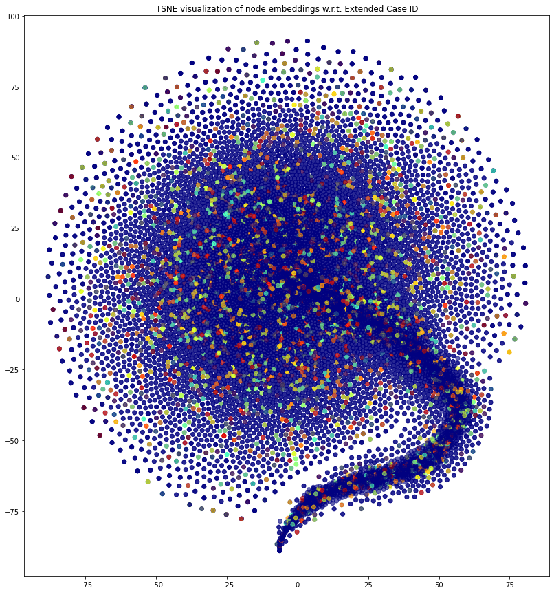
Figure 1. Homogeneous (subsampled) graph embeddings with Deep Walk. Coloring on ExtendedCaseGraphID. You can see that the nodes are all clustered together.

3.2. Metapath2Vec

This is a variation of DeepWalk. It uses metapath definitions to navigate the random walks and creates a corpus that is used with the same techniques as DeepWalk. You can clearly see a step forward, but the graph is still treated as homogeneous and the nodes are not really separated in communities.

Figure 2. Homogeneous graph embeddings with Metapath2Vec. Coloring on ExtendedCaseGraphID. I've achieved some separation but not something meaningful.

3.3. MAGNN (Metapath Aggregated Graph Neural Network for Heterogeneous Graph Embeddings)

I found the Aggregated Metapath strategy really interesting, but I couldn’t make it work on my dataset, because I didn’t find any documentation on the preprocessing pipeline used by the authors. In the end, I still believe this wouldn’t have been a good approach, because metapaths are limited. With that I mean that different metapaths convey different semantic meanings, but MAGNN ignores the preferences of nodes on different metapaths. Still, it would’ve been interesting to compare its embedding capability on this dataset.

3.4. HAN (Heterogeneous graph Attention Network)

The paper for this approach is very promising and this model outperforms most of the other techniques. However, it has one deal breaker: in order to preprocess the data for HAN, according to its authors “you must extract balanced node labels, which means different classes should have almost the same number of nodes. For k classes, each class should select 500 nodes and label them, so we get 500*k labeled nodes”. Unfortunately, my graph has severely imbalanced classes with regard to CoreCaseGraphID and ExtendedCaseGraphID, with many classes having as little as 1 sample only, as stated in the 2.1 section.

3.5. HinSAGE

This is the heterogeneous version of GraphSAGE. It has all the advantages of the latter, and is offered as implementation in the stellargraph library (although with only one kind of aggregator, mean-pooling). Being similar to GraphSAGE, HinSAGE should allow me to use the trained model on new nodes that it has never seen before, to create embeddings “on the fly”. It checks all the boxes for an ideal model for this task. I used it in many different ways, both with end-to-end training (by adding a keras Dense layer) and with the unsupervised Deep Graph Infomax technique.

I decided to focus on the heterogeneous graph methods instead of splitting the dataset into homogeneous subgraphs to be able to use homogeneous graph techniques, since I didn’t want to lose too much information on an already complicated scenario. Apparently there are ways to split a heteogeneous information graph into homogeneous subsets with APPNP (Approximate Personalized Propagation of Neural Predictions) or with HGT (Heterogeneous Graph Transformer). It would be extremely interesting to investigate the quality of such methods, but I ended up focusing on HinSAGE because of time constraints.

3.5.1. End-to-end HinSAGE

I used two HinSAGE layers for embedding and one keras Dense layer for node inference, trained end to end to minimize a global cost function. Initially I thought this approach would be more robust for class imbalance, but this turned out not to be the case. In fact, the results were very disappointing: at first glance, the model converged by predicting all extended cases to 0, since it was the most imbalanced class.

Practically, the model found a local minimum by predicting all 0’s, and the accuracy remained the same from the 3rd epoch onward. This is also very easy to diagnose by looking at the learning curves (the loss appears flat). To be fair, the accuracy score obtained by predicting all 0’s was about 30% which is not bad, but accuracy tells us very little about the prediction quality for this task - this is why we use F1 score in the first place.

The only improvement I made to this model was to create a class weight dictionary and pass it to the fit method. This way I could control how much weight the model gave to any specific sample. I used it to reduce the weight of the label class 0 (corresponding to ExtendedCaseGraphID=0), so the model needed to find different local optima. Nonetheless, even with this improvement, the model performed poorly, so I decided to try an unsupervised (or semi-supervised) method and train an embedding model and a node classification model separately to have more granular control. You can still see this method in the Notebook: ”HinSAGE E2E”.

3.5.2. Unsupervised HinSAGE with Deep Graph Infomax

I trained a HinSAGE embedding model with the unsupervised Deep Graph Infomax method, and then fed the embeddings as input to a classifier to predict the ExtendedCaseGraphID. I must say that the Deep Graph Infomax method captured my attention like no others during this contest. By reading the official paper of this approach I was astounded by the results obtained considering that it’s semi-supervised.

DGI is a procedure for training all kinds of graph ML models without supervision. It trains a model to capture patterns in the connections between nodes and their features by checking “true” nodes against a corrupted version. This method can be used both as initialization or pre-training when some labeled data are available, like in this case. Nonetheless, I decided to try it and to my surprise it was very fast to run, so I could run it across the entire graph, with all my node and edge types, my custom features, the edge weights and so on. It was the only method I found that had no limitations regarding class imbalance, data quality or anything else.

One note on the HinSAGE model in general: it can leverage the whole heterogeneous graph for training, but it can make predictions on one node type at a time, so I had to run it for each node type.

This was a problem because I then needed to make adjustments on some parameters, namely the layer sizes and activations. I ran into some dimensionality issues while trying to run HinSAGE layers on smaller node types like External Entity and Address. Due to time restrictions I decided to run the model only on Account, Customer and Derived Entity nodes. As stated in section 2.1, this still gave me 80% of the labeled cases so I ended up discarding the External Entity and Address nodes for predictions.

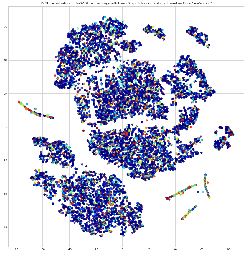
Figure 3. HinSAGE DGI Account embeddings of testingFlag=0 nodes. Colored on CoreCaseGraphID. 15 epochs.

4. Result quality considerations

In this section I want to explain why I believe the embeddings I obtained from the last method, HinSAGE with DGI (section 3.5.2), are of good quality.

Node Embeddings are a reflection of the features and the connections in the graph. As such, a good embedding is a map that goes from the actual node in the graph to a n-dimensional vector in such a way that the characteristics of each node are translated in the embedded vector. For example, far away nodes that have no connections between them should have very different embeddings, and similar nodes should have similar embeddings.

This begs some questions: How much does each feature of each node weight in the final embedding? And most importantly: How do I evaluate similarity between nodes? There are many different notions of similarity and one is not better than the others. For example, there are adjacency-based similarities (e.g. nodes are similar if they’re connected), multi-hop similarity, random walk approaches, and more. There’s even the ”is similar” edge type that could be weighted in the optimal notion of similarity for this dataset.

Since in my solution I’m using HinSAGE, which is GraphSAGE in its core, I know that it has a context-based similarity assumption. In other words, GraphSAGE assumes that nodes that reside in the same neighborhood should have similar embeddings. This definition is also parametric with a parameter K denoting the depth at which it considers a node to be part of its neighborhood.

Since I used the Stellargraph implementation of this algorithm, I wasn’t able to find a quick way to change the K parameter for testing. I believe that this parameter could have a huge delta in embedding quality. I’ve thought about building a custom implementation of GraphSAGE with Pytorch for this reason alone, but I ended up discarding the idea.

5. Future improvements

During the contest I thought about some different ways that I could have framed the task. In particular, I’m not sure that the node embedding model alone is the best solution here. The methods I’m going to describe here aren’t tested and may not work, but I’d be interested in trying them:

• I could use a global overlap measure on all nodes, and a local overlap measure on the nodes with the same CoreCaseGraphID. It could be possible to detect communities by confronting the local & global overlaps. For instance, if all the nodes with CoreCaseGraphID=305 have a similar overlap to one specific node, this node may be part of the same case.

• It would be very insightful to use a graph visualisation tool such as Stellargraph Visualisation, to get a concrete look at the graph and understand it better. Unfortunately such software is proprietary and only sold to enterprises (as far as I know).

• By building a custom implementation of GraphSAGE, I could use a different notion of similarity (other than context-based). For example I could add a value representing the weight of the ”is similar” out-going and in-going edges for each node, or a value representing the adjacency to fraudulent nodes (aka nodes with a CoreCaseGraphID).

• Another approach could be to use a clustering technique like Cluster-GCN, and use a custom clustering function (like the METIS algorithm) to create 4000 different clusters corresponding to the Core Cases and use neural network layers on that.

6. Conclusion

In summary, in this report I explained how I framed the task for my solution, I showed how I analysed the dataset and its features, I experimented a lot with different embedding methods and finally I proposed my submission, composed of HinSAGE trained with Deep Graph Infomax and a Decision Tree classifier. Finally I explained why the results didn’t meet a satisfactory score and I went through all the ways in which my solution could be improved.

7. Acknowledgements

A big thank you to NECSTLab and Oracle Labs for running this contest: like I said, this has been the most challenging event of my academic life so far and a huge learning opportunity.

If you really read this until the end, thank you so much for your attention. If you want to get in touch with me, feel free to send me an email.